Probablity & Statistics
Last updated: 28 Oct 2025
Basics
-
Experiment : Repeatable task with well defined outcomes
-
Sample Space : All possible outcomes of an experiment
-
Event : A subset of sample space of experiment $E\subseteq S$
Set Theory
- $\ A \subseteq B => A\ subset\ of\ B $
- $\ A = B => A\subseteq B \ and \ B\subseteq A$
- Empty set ($\phi$) => Set with no element => $\phi$ is contained in every set
Operations with sets
$A\cup B = { x: x \in A\ or\ x \in B }$
$A\cap B = { x: x \in A\ and \ x \in B }$
$A^c = { x : x\notin A }$
Suppose we have an $\Gamma$ be indexing set and we have {$A_\alpha ,\ \alpha \in \Gamma$} be collection of sets indexed by $\Gamma$
then , $\bigcup\limits_{\alpha\in\Gamma} A_\alpha = { x : x \in A_\alpha\ for\ some\ \alpha \in \Gamma}$
and $\bigcap\limits_{\alpha\in\Gamma} A_\alpha = { x : x \in A_\alpha\ for\ every\ \alpha \in \Gamma}$
-
A and B are disjoint if $A \cap B = \phi$, A and B are Mutually Exclusive
-
$A_1, A_2, ..... $ are pairwise disjoint if $A_i \cap A_j = \phi \qquad \forall\ i \neq j$
-
$A_1, A_2, ..... $ is a partition of S if :
-
$A_1, A_2,...$ are pairwise disjoint
-
$\bigcup\limits_{i} A_i = S$
-
Sigma Algebra
-
Collection of subsets of S
-
Satisfying
-
$\phi \in \mathcal{B}$
-
if $A \in \mathcal{B},\ then\ A^c \in \mathcal{B}$
-
if $A_1, A_2, A_3,... \in \mathcal{B}$, then $\bigcup\limits_{i=1}\limits^{\infty} A_i \in \mathcal{B}$, (closed under countable unions).
-
-
${\phi, S}$ is trivial sigma algebra associated with S.
Probablity Function
-
Probablity function for pair (S, $\mathcal{B}$) is defined for P:$\mathcal{B}\ \rightarrow \mathbb{R} $ if it satisfies below Axioms of Probablity:
-
$P(A) \geq 0 \qquad \forall A\in \mathcal{B}$
-
P(S) = 1
-
if $A_1, A_2, A_3,... \in \mathcal{B}$, are pairwise disjoint (countable) then $P(\bigcup\limits_{i=1}\limits^{\infty}) = \sum\limits_{i=1}\limits^{\infty}P(A_i) $)
-
-
Properties of Probablity fn :
-
P($\phi$) = 0
-
P(A) $\le$ 1
-
P($A^c$) = 1 - P(A)
-
0 $\le P(A) \le$ 1
-
$P(B\cap A^c) = P(B) - P(A\cap B)$
-
$P(A \cup B) $ = $P(A) + P(B) - P(A\cup B)$
-
if $A \subseteq B$ => P(A) $\le$ P(B)
-
Conditional Probablity & Independence
-
Conditional P : Decision under influence of info
-
P(A|B) = Probablity of A given B has occured
-
$P(A|B) = \frac{P(A\ \cap\ B)}{P(B)}$
-
Multiplication Rule : $P(A\cap B) $ = $P(A|B)\cdot P(B) $ = $P(B|A)\cdot P(A)$
-
Independent Events : $A, B \subseteq S$ are independent iff
- $P(A|B) = P(A),$ and $P(B|A) = P(B)$
Bayes Theorum
-
use prior probablities to calculate posterior probablities
-
$P(A_j | B) = \frac{P(B|A_j) \cdot P(A_j)}{\sum\limits_{i-1}\limits^{n} P(B|A_i) \cdot P(A_i)} $, all probablities on rhs are prior probs
Counting
-
Fundamental Theory of Counting
-
Let T be task of perfoming k tasks sequentially : $T_1, T_2,....T_k$ that can be permormed in $n_1, n_2,....n_k$ ways,
-
Total no of ways to perform T = $n_1\cdot n_2...\cdot n_k$
-
| \ | Without Replacement | With Replacement |
|---|---|---|
| Ordered | ${}^nP_k = \frac{n!}{(n-1)!}$ | $n^k$ |
| Unordered | ${}^nC_k = \frac{n!}{(n-k)!\ *\ k!}$ | ${}^{n+k-1}C_k$ |
Random Variables
-
If S is sample space of an experiment, Random Variable X is a function whose domain is S and range a new sample space.
$X: S \rightarrow \mathbb R$
$w \rightarrow X(w)$ -
Image of X : X(S) = values of X on outcomes in S. [new sample space for original experiment]
-
If ${X=c} \subseteq S$ form a partition of S, then $S=\bigcup\limits_{c \in X} {X=c}$ (Disjoint union)
-
Probablity distribution table for X looks like below:
| $x\in \chi$ | 0 | 1 | 2 | 3 | 4 |
|---|---|---|---|---|---|
| P(X=$x$) | 1/16 | 4/16 | 6/16 | 4/16 | 1/16 |
- Note that sum is 1, hence partition of samples space.
Probablity Distribution of Random Variables
-
for X : S -> R, the values $\chi$ of X define a new sample space.
-
if P is probablity fn for S, this induces a probablity fn for X : $P_X$ on $\chi$
-
Cumulative distribution fn of X : $F_X(x) = P(X\le x),\ \forall x$
-
A fn F(x) is cdf iff it follows the 3 conditions:
-
$\lim\limits_{x\rightarrow -\infty} F(x) = 0, \quad \lim\limits_{x\rightarrow +\infty} F(x) = 1$
-
F(x) is a non-decreasing fn.
-
F(x) is right continuous, i.e. $\lim\limits_{x\rightarrow x_0^+} F(x) = F(x_0), \quad \forall x_0 \in \mathbb R$
-
| X is Discrete | X is Continuous |
|---|---|
| $F_X(x)$ is step fn | $F_X(x)$ is continuous fn |
| Probablity Mass fn pmf is $p_X(x) = P(X=x),\ \forall x$ | Probablity density fn pdf is $F_X(x) = \int\limits_{-\infty}\limits^x f_X(t)\ dt,\ \forall x$ |
| $\chi$ is discrete subset of $\mathbb R$. | $\chi$ is a union of intervals in $\mathbb R$. |
| CDF: $F_X(x) = P(X\le x) = \sum\limits_{y\in \chi,\ y\le x} p_X(y)$ | CDF : $F_X(x) $ = $P(X\le x) $ = $\int\limits_{-\infty}\limits^x f_X(t) dt$ |
| $P(a\le X \le b) = F(b) - F(a^-)$ $a^-$ is largest possible val of X strictly less than a |
$P(a \le X \le b) $ = $\int\limits_a\limits^b f_X(x) dx$ = $F_X(b) - F_X(a)$ |
NOTE :
-
if X is discrete with $c\in \chi,\qquad P(X=c) = p_X(c)$,
-
if X is continuous $P(X=c) = P(c\le X\le c) $ = $\int_c^cf_X(x) dx = 0$
Expectation of Random Variables
-
if discrete : $E(X)$ or $\mu_x = \sum\limits_{x\in\chi} x.p_X(x)$
-
if continuous : $E(X) = \int_{-\infty}^\infty x.f_X(x)\ dx$
-
similar if h(X) is fn of X, replace X with h(x) in LHS and x with h(x) in RHS.
Variance of Random Variable
-
V(X) or $\mu_X^2 = E[(X-\mu_X)^2]$
-
if Discrete : V(X) or $\sigma_X^2 = \sum\limits_{x\in \chi} (x-\mu_X)^2.\ p_X(x)$
-
if continuous : $V(X) = \int_{-\infty}^{\infty} (x-\mu_X)^2.f_X(x) \ dx$
-
Standard Deviation $\sigma_X = \sqrt{V(x)}$
Properties of Expectation and Variance
-
if X is scaled to ax+b, E[h(x)] = E[aX+b] = aE(x) + b
-
V[h(X)] = $a^2$V(X) and SD(h(x)) = |a|SD(x)
-
$V(X) = E(X^2) - (E(X)^2)$
Continuous Random Variable
- if X is continuous random var and $f_X$ is pdf of X, then cdf $F_X$ is continuous function
$F_X(x) =P(X\le x) $ = $\int_{-\infty}^x f_X(t) \ dt$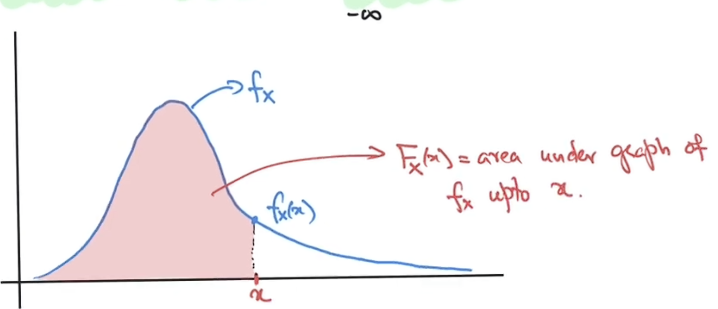
-
$P(a \le X \le b) $ = $ \int\limits_a\limits^b f_X(x) dx $ = $F_X(b) - F_X(a)$
-
$P(X=c) = F_X(c) - F_X(c) = 0$, continuous random var cannot take a particular val.
-
$P(X \gt c) = 1 = P(X \le c) = 1-F_X(c)$
-
We can use cdf to calculate pdf : $f_X(x) = F_X'(x)$
-
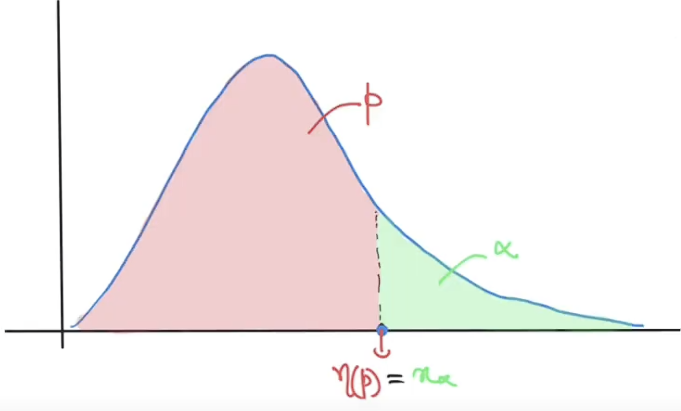
Let p in (0,1), the (100*p) th percentile for the distribution of X : $\eta(p)$ satisfies
$p=F_X(\eta(p)) = \int\limits_{-\infty}\limits^{\eta(p)}f_X(x)\ dx$ -
Let $\alpha$ in (0,1), the $\alpha^{th}$ critical val for the distribution of X : $x_\alpha$ satisfies
$\alpha = P(X>x_\alpha) = 1-F_X(x_\alpha)$
-
Note : (100*p)th percentile - same as -> 100(1-p)th critical value
Discrete Random Variables
-
given cdf of X as "$F_X$" and pdf of X as "$f_X$" or "$p_X$" ,
-
X is discrete if cdf $F_X$ is a step fn.
-
When X is discrete, $\chi$ will be discrete subset of $\mathbb R$ and will be:
-
finite set : in bijection with {1,2,3,....... n} for $n\in \mathbb N$
-
countably infinite set : in bijection with $\mathbb N$
Below are the different discrete random variables with finite $\chi$
-
-
Uniform Discrete RV
-
$p_X(x) = P(X=x) = \frac{1}{N}$
-
E(X) = $\frac{N+1}{2}$
-
V(X) = $\frac{N^2-1}{12}$
-
Calculation of $p_X(x) = P(X=x)$ depends on if
-
Sampling without replacement => Hypergeometric distribution with params : N, M, n
-
Sampling with replacement => Binomial distribution with params : n, p=M/N
-
Hypergeometric Distribution
-
P(X=x) = P( getting "x" successes in a sample of size "n" sampled without replacement from population of N size with M successes )
-
$p_X(x) = \frac{(^M_x)\ \ (^{N-M}_{n-x})}{(^N_n)}$
-
E(X) = $\frac{nM}{N}$ = np (if p = M/N)
-
V(X) = $\frac{n(N-n)}{N-1}\ p\ (1-p)$ if p=M/N
-
-
Binomial Distribution
-
$p_X(x) = (^n_x)\ p^x\ (1-p)^{n-x}$
-
E(X) = np
-
V(X) = npq
-
-
Bernoulli Distribution
-
success = p, failure = 1-p, single try.
-
E(X) = p
-
V(X) = p(1-p)
Below are Different discrete variables with infinite $\chi$ :
-
-
Poisson's Distribution
-
$p_X(x) = \frac{e^{-\lambda} \cdot \lambda^x}{x!} \qquad where\ e^\lambda= 1+\lambda + \frac{\lambda^2}{2!} + \frac{\lambda^3}{3!} + .....$
-
we assume $p_X(x) \ge 0$ for legitimate PMF
-
$E(X) = \lambda$
-
$V(X) = \lambda$
-
-
Negative Binomial Distribution
-
Do repeated trials with P(success) = p till r success are observed with x failures
-
$p_X(x) = (^{x+r-1}x) \cdot p^r \cdot (1-p)^x $ = $(^{n-1}{n-r}) \cdot p^{n-x} \cdot (1-p)^{n-r}$ in terms of n; n=x+r
-
E(X) = $\frac{r(1-p)}{p}$
-
V(X) = $\frac{r(1-p)}{p^2}$
-
-
Geometric Distribution
-
Repeatedly do trials till one success.
-
Its special case of negative binomial pmf with r=1.
-
$p_X(x) = p(1-p)^{x-1}$
-
$E(X) = \frac{1}{p}$
-
$V(X) = \frac{(1-p)}{p^2}$
-
NOTE :
-
if $ N,M \rightarrow \infty\ $ such that$\frac{M}{N} \rightarrow p : hypergeometric(x;N,M,n) \rightarrow binomial(x;n,p) $
-
if $n\rightarrow \infty\ and \ p\rightarrow0\ $ such that $np\rightarrow\lambda : binomial(x;n,p) $ $ \rightarrow poissons(x;\lambda)$
-
Uniform Continuous Dist - Cont Rand Variable
-
PDF : $f(x) = 1/(B-A) \quad x\in [A,B],$ 0 otherwise
-
CDF : $F(x) = x/(B-A)\quad if\ x\in [A,B]$ $,0\ \ if\ x<A,\ 1\ \ if\ x\ge B$
-
E(X) = (B+A)/2
-
V(X) = $\frac{(b-a)^2}{12}$ where a,b in [A,B] and a<b
Normal Distribution - Continuous Random Variable
-
Denoted by $N(\mu, \sigma^2)$: mean $\mu$ and variance $\sigma^2$.
-
if X is normally distributed, pdf of X : $f(x) = \frac{1}{\sqrt{2\pi}\sigma} \cdot e^\frac{-(x-\mu)^2}{2\sigma^2} \quad x\in(-\infty, \infty)$
-
CDF : $F_X(x) = P(X\le x) $ = $ \int\limits^x_{-\infty}f(t)dt = \frac{1}{\sqrt{2\pi}\sigma} \int\limits_{-\infty}^x e^\frac{-(t-\mu)^2}{2\sigma^2}dt$
make integrals from a => b to calculate P( a <= X <= b) -
Standard Normal Distribution : normal dist where N(0, 1) i.e. mean = 0, variance = 1
-
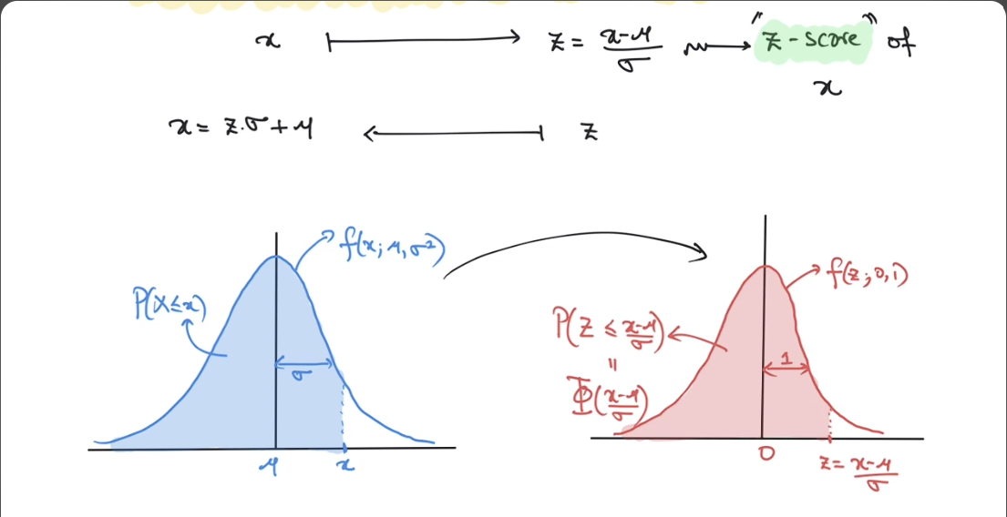
if X is normal distribution $N(\mu, \sigma^2)$ and Z is standard normal distribution $Z\sim N(0,1)$
$\qquad P(X\le x) = \frac{1}{\sqrt{2\pi}\sigma} \int\limits_{-\infty}^x e^\frac{-(t-\mu)^2}{2\sigma^2} dt$
let $s = \frac{t-\mu}{\sigma}$
$\qquad P(X\le x) = \frac{1}{\sqrt{2\pi}} \int\limits_{-\infty}^\frac{x-\mu}{\sigma} e^\frac{-s ^2}{2}ds = P(Z\le\frac{x-\mu}{\sigma})$
This Denotes $X\sim N(\mu, \sigma^2)$ then $(x-\mu)/\sigma$ has the standard normal distribution -
$z = (x-\mu)/\sigma$ is called as Z-score of x
-
cdf of normal distribution is often denoted by $\Phi(z)$
-
if Z is standard normal dist and $z_\alpha$ is $\alpha^{th}$ critical value , then it satisfies
$P(Z\ge z_\alpha) = \alpha \text{}$
$1-P(Z\le z_\alpha) = 1-\Phi(z_\alpha) = \alpha$ -
if $p \in (0,1)$, (100p)th percentile, $\eta (p)$ satisfies
$P(Z\le \eta(p)) = \Phi(\eta(p)) = p$ -
Suppose $X\sim N(\mu, \sigma^2)$ and $\alpha \in (0,1)$
$\alpha$th critical value = $x_\alpha = \sigma \cdot z_\alpha + \mu$ where $\ z_\alpha = \alpha \text{th critical value for } Z \sim N(0,1 )$Approximate Bin(n,p) using Normal Distribution
- Let $X \sim Bin(n,p)$ where $ \mu_X = np\ \quad \sigma^2 = npq$
if Bin(n,p) is not too skewed,
$P(X\le x) \approx \Phi((x+0.5-\mu_X)/\sigma_X)$
Gamma Distribution - Continuous Random Variable
-
Useful when modelling events related to time, eg component lifetimes, waiting times, etc.
-
Gamma fn $\Gamma(\alpha) = \int_0^\infty t^{\alpha-1} e^{-t}dt$, for $\alpha > 0$
-
Properties :
-
$\Gamma(\alpha) = \alpha\ \Gamma(\alpha)$
can check if $\Gamma(1) = 1$ and using induction we have $\Gamma(n) = (n-1)!$ -
$\Gamma(1/2) = \sqrt{\pi}$
-
$f(x; \alpha, \beta) = \frac{1}{\beta^\alpha\ \Gamma(\alpha)} \cdot x^{\alpha-1} \cdot e^{-x/\beta}$ if x>=0, else 0
we note below:-
$f(x;\alpha, \beta) \ge 0 \quad \forall x\in \mathbb R$
-
$\int^\infty_{-\infty} f(x; \alpha, \beta) dx = 1$
f will be pdf of given variable
-
-
-
We can say X has gamma dist with shape param $\alpha$ , and scale param $\beta$ if the pdf of X is $f(x; \alpha, \beta)$
-
when beta = 1 => "Standard Gamma distribution" wiht shap param $\alpha$
-
if X ~Gamma(alpha, beta) then
-
E(X) = $\mu_X = \alpha \cdot \beta$
-
V(X) = $\sigma_X^2 = \alpha \cdot \beta^2$
-
$ \sigma_X = \sqrt{\alpha} \cdot \beta$
-
-
The cdf of X ~ Gamma(alpha, beta)
$F_X(x; \alpha, \beta) = \int_0^x f(t; \alpha, \beta)\ dt$ if x>0, 0 otherwise -
$P(X \le x) = F_X(x; \alpha, \beta) = F(x/\beta; \alpha)$ [cdf of standard gamma with param $\alpha$]
-
if T has standard gamma with shap param $\alpha$ => X = $\beta \cdot T$ has gamma dist with shape alpha and scale beta
-
Special cases of Gamma Distribution
-
Exponential dist : $\alpha = 1,\ \beta = 1/\lambda$
-
Get exponential dist with param $\lambda > 0$
-
pdf $f(x; \lambda) = \lambda \cdot e^{-\lambda x}$ if x>=0, 0 otherwise
-
cdf $F_X(x; \lambda = 1-e^{-\lambda x}$
-
$E(X) = \mu_X = 1/\lambda$
-
$V(X) = \sigma_X^2 = 1/\lambda^2$
Poisson process with rate $\alpha$ => the exponential dist with $\lambda = \alpha$ models the distribution of elapsed time b/w occurence of 2 successive events
if X ~ Exp($\lambda$) : $P(X \ge t+t_0\ |\ X \ge t_0)$ = $\frac{P[(X \ge t+t_0) \cap (X\ge t_0)]}{P(X \ge t_0)}$ = P(X>=t)
-
-
Chi-Squared Dist: X ~ Gamma (alpha, beta) with $\alpha = v/2,\ \beta = 2$
-
param is $v$ : degrees of freedom
-
pdf $f(x; v) = (x^{v/2 - 1} \cdot e^{-x/2}) / (2^{v/2} \cdot \Gamma(v/2))$ if x >=0, 0 otherwise
-
$E(X) = \mu_X = \alpha \cdot \beta = v$
-
$V(X) = \sigma_X^2 = \alpha \cdot \beta^2 = 2v$
-
chi-square dist is imp in statistical inference of population variance
-
if $X\sim N(\mu, \sigma^2)$ then $(\frac{x-\mu}{\sigma})^2$ has chi-sq dist with v=1
-
-
Log Normal Dist - CRV
-
X has log normal dist if ln(X) has normal dist : $ln(X) \sim N(\mu, \sigma^2)$
-
if X has lognormal dist, pdf $f(x; \mu, \sigma) = $ $\frac{1}{\sqrt{2\pi}\sigma} \cdot e^{-(ln(x)-\mu)^2/2\sigma^2}$ if x >=0 , 0 otherwise
Note $\mu \text{ and } \sigma$ are mean and variance of ln(X) -
E(X) = $\mu_X = e^{\mu +\sigma^2/2}$
-
V(X) = $\sigma_X^2 = e^{2\mu + \sigma^2}(e^{\sigma^2} - 1)$
-
to use std normal dist to calc probablities
cdf $F_X(x; \mu, \sigma) =$ $P(X \le x) = \phi(\frac{ln(x) - \mu}{\sigma})$
Beta Dist
-
takes vals in finite interval
-
X is said to have beta dist with param $\alpha, \beta > 0$ if pdf of X is
$F(x; \alpha, \beta) =$ $\frac{\Gamma(\alpha + \beta)}{\Gamma(\alpha)\cdot \Gamma(\beta)} \cdot x^{\alpha-1} \cdot (1-x)^{\beta-1}$ where x in (0,1) -
called beta dist because of beta fn $B(\alpha, \beta) = \frac{\Gamma(\alpha)\cdot \Gamma(\beta)}{\Gamma(\alpha + \beta)}$
-
E(X) = $\mu_X = \frac{\alpha}{\alpha + \beta}$
-
V(X) = $\sigma_X^2 = \frac{\alpha \beta}{(\alpha+\beta)^2 (\alpha + \beta+1)}$
-
Depending on values of alpha and beta, pdf has diff shapes:
-
alpha > 1, beta = 1 => strictly increasing
-
alpha = 1, beta > 1 => strictly decreasing
-
alpha < 1, beta < 1 => U shaped
-
alpha = beta => symmetric about 1/2, with $\mu_X = 1/2$ and $\sigma_X^2 = 1/4(2\alpha+1)$
-
alpha = beta = 1 => get uniform dist on (0,1)
-
Cauchy Dist
-
X is said to have cauchy dist with param $\theta$ if
pdf(X) = $f(x; \theta) = \frac{1}{\pi(1+(x-\theta)^2)}$ -
E(X) and V(X) do not exists for cauchy dist
-
graph of pdf is bell shaped (like normal density) but has heavier tails
-
Related to t-distribution