Back to Home
Last updated : 10 Oct 2025

ML Basics

• ML is study of of algo that Improve on task T, wrt performance metric P, based on experience E

• ML categories are

  1. Classification
  2. Generation
  3. Novelty detection

• ML Algorithms:

  1. Nearest Neighbour
  2. Naive Bayes
  3. Decision Trees
  4. Linear Regression
  5. Support Vector Machines (SVM)
  6. Neural Networks

• Deep learning is specialised area within ML concerned with neural networks.

• Types of learning in ML Systems :

  • Supervised :
    Given Training Data + labels
    Used when abundant labeled data

  • Unsupervised :
    Given training data without labels
    goal is to discover hidden structures or patterns
    Used when we want to explore structure in raw data
    eg : clustering, dimensionality reduction (t-SNE or PCA), ICA

  • Semi-supervised :
    combines supervised and unsupervised
    given training data + few labels
    Used in common real world scenario where labelling is expensive or time consuming.

  • Reinforcement :
    Agent interacts with environment
    Given seq of states & actions with rewards (delayed) & penalties
    output a policy or mapping from states action that tells what to do in given state (maximize cumulative reward).
    Used when learning is based on interaction and delayed rewards.
    eg. playing super mario game:

    • Rewards - collecting coins, defeating enemies, completing levels

    • Penalties - falling in pit, running out of time

Bayesian Decision Theory

• Bayes Theory : Converts class prior P(wi) and class conditional densities p(x|wi) to posterior probablity for a class P(wi|x).
  P(w_i|x) = \frac{p(x|w_i)*P(w_i)}{p(x)} \qquad$P(w_i|x) = \frac{p(x|w_i)*P(w_i)}{p(x)} \qquad$
  where,
  posterior = (likelihood x prior) / evidence
  Posterior probablity P$P$ : updated belief after observing data
  Prior probablity p$p$ : belief before observing data

• Bayes Decision Theory : to minimize errors, chose the action/class that minimizes expected loss (i.e. Select lease risky class).

• Decision function \alpha(x)$\alpha(x)$ : Rule for making decision. Feature vector x \rightarrow$x \rightarrow$ action/class \alpha(x)$\alpha(x)$

• Risk Function R : Expected loss of (after) making each decision
  R = \int R(\alpha_i|x) p(x)\ dx$R = \int R(\alpha_i|x) p(x)\ dx$ ,
  where R(\alpha_i|x) = \sum\limits_{j=1}\limits^{n} \lambda_{ij}\ P(w_j|x) \qquad$R(\alpha_i|x) = \sum\limits_{j=1}\limits^{n} \lambda_{ij}\ P(w_j|x) \qquad$ and \lambda$\lambda$ is loss function
  \lambda(a_i|w_j) = \lambda_{ij}$\lambda(a_i|w_j) = \lambda_{ij}$ is cost of selecting class i when sample belongs to class j

• Goal of Bayesian decision theory: choose class i if : \quad R(\alpha_j|x) \le R(\alpha_j|x) \qquad \forall j\ne i$\quad R(\alpha_j|x) \le R(\alpha_j|x) \qquad \forall j\ne i$

• Note:

  • if data is Discrete Random variable, eg rolling fair die - 1,2,3,4,5,6
    use Probablity Mass Function (PMF).

  • if its Continuous Random Variable i.e. any value b/w range/interval
    eg : exact weight of person, x in [0,180]
    use Probablity Density Function (PDF)

  • Class-Conditional Probablity p(x|w)$p(x|w)$ : The probablity of observing a certaain input feature x$x$, given it belongs to specific class w$w$
    Bayes formula convert class prior P(w_i)$P(w_i)$ and class-conditional probablity p(x|w_i)$p(x|w_i)$ to posterior probablity for class P(w_i|x)$P(w_i|x)$.

Bayesial Classifier Decision

Discriminant Fn g_i(x)$g_i(x)$:

• Helps classifier decide which class to assign to given input.

• Example :

  • General Discriminant fn : g_i(x) = -R(\alpha_i|x)$g_i(x) = -R(\alpha_i|x)$

  • Zero-One loss discriminant fn : g_i(x) = P(w_i|x)$g_i(x) = P(w_i|x)$

• Decision : Decide class 'i' if, g_i(x) \ge g_j(x) \quad \forall i \ne j$g_i(x) \ge g_j(x) \quad \forall i \ne j$

Equivalent Discriminants for Zero-One loss :

• all classification errors are treated equally

• \lambda(\alpha_i | w_j) = \begin{cases} 0 & \text{if } i=j \\ 1 & \text{if } i\ne j \end{cases}$\lambda(\alpha_i | w_j) = \begin{cases} 0 & \text{if } i=j \\ 1 & \text{if } i\ne j \end{cases}$

• Decision : choose class that maximizes posterior probablity

Decision Region for Binary classifier : The boundary b/w regions where discriminant fn is equal for the 2 classes

Gaussian (Normal) Distribution

Plays major role in many bayesian classifier. Types are :

1. Univariate Normal Distribution models a single continuous variable (eg. height, temp)

2. Multivariate Normal Distribution models multiple features together.

Key variables : mean \mu$\mu$, variance \sigma^2$\sigma^2$, covariance matrix \Sigma$\Sigma$.

Maximum Likelihood Estimation (MLE)

• MLW and MAP help infer most plausible params for models based on available evidence.

• Goal : Choose model parameters that make observed data as likely as possible.

• Likelihood fn p(D|\theta)$p(D|\theta)$ measures how likely observed data is for diff param vals.

• Let dataset D contain n samples p(D|\theta) = \prod\limits_{k=1}\limits^n p(x_k|\theta)$p(D|\theta) = \prod\limits_{k=1}\limits^n p(x_k|\theta)$
  having natural log for likelihood, called Log-Likelihood
  \ln(\theta) = \ln p(D|\theta) = \sum\limits_{k=1}\limits^n \ln p(x_k|\theta)$\ln(\theta) = \ln p(D|\theta) = \sum\limits_{k=1}\limits^n \ln p(x_k|\theta)$
  \frac{d}{d\theta} \ln (\theta) = \sum\limits_{k=1}\limits^n \frac{d}{d\theta} \ln p(x_k|\theta)$\frac{d}{d\theta} \ln (\theta) = \sum\limits_{k=1}\limits^n \frac{d}{d\theta} \ln p(x_k|\theta)$
  set $\frac{d}{d\theta} \ln(\theta) = 0 $ and solve for params

• Below is comparision of MLE vs Bayesian Estimate

  Max Likelihood Est (MLE)	Bayesian Estimate
  Views the params as fixed but unknown vals	Views params as random vars with some known prior distributions
  Best estimate is one that maximizes likelihood of data	Update beliefs after observing data.

• As data grows, In Bayesian setting:

  • Prior influence decreases

  • Posterior influence increases around MLE solution

• So Bayesian estimate and MLE converge to same sample in large dataset.

Maximum Posterior Estimation (MAP)

• Goal : Maximizing posterior Probablity of prams in given observed data.

• Combines MLE and Bayesian estimate.

• If we assume uniform prior influence, MAP is same as MLE.

• Usecases :

  • More Data (no strong Priors) -> MLE

  • Less Data (less strong priors) -> Bayesian or MAP

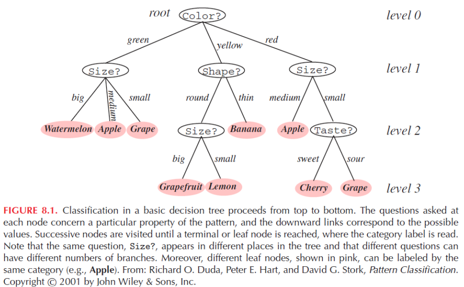
Decision Trees

• Each internal node asks question about feature, each branch corresponds to possible answer & each leaf node is prediction.

• Decision tree can represent any boolean functions

• UseCase :

  • Model needs to be easy to interpret.

  • Can handle both categorical & numerical data

  • Naturally incorporate feature interactions.

• Overfitting:

  • Caused when decision tree is Too Deep or Too Often Splits

  • Model learns more noise than actual data.

  • Leads to poor performance on unseen data.

• Its very expensive with more nodes, Always try to make small tree.

• Metrics for Splitting Criterion:

  • Info Gain : Choose Split that reduces uncertainty.

  • Accuracy BAsed : Choose split that gives highest accuracy for immediate classification

  • Gini Impurity : Fast calculation or less concern for interpretablity (popular for Real-time system or large scale classification)

Info Gain

Measures how much feature tells about class label:

I(X,Y) = H(X) - H(X|Y)$I(X,Y) = H(X) - H(X|Y)$ = H(Y) - H(Y|X)$H(Y) - H(Y|X)$

where,

Entropy for x: H(X) = -\sum\limits_{i=1}\limits^n P(x=i) \log_2P(X=i)$H(X) = -\sum\limits_{i=1}\limits^n P(x=i) \log_2P(X=i)$
H(X|Y=v)$H(X|Y=v)$ = -\sum\limits_{i=1}\limits^n P(x=i|Y=v) \log_2P(X=i|Y=v) H(X|Y) = \sum\limits_{v\in Y} P(Y=v) \cdot H(X|Y=v)$-\sum\limits_{i=1}\limits^n P(x=i|Y=v) \log_2P(X=i|Y=v) H(X|Y) = \sum\limits_{v\in Y} P(Y=v) \cdot H(X|Y=v)$

Note : To prevent Overfitting -

1. Limit tree depth

2. set min no of samples req for splitting node.

3. use cross validation.

Steps to create Decision Tree :

1. Calc entropy for entire Dataset
   H(S) = -\sum\limits_{i=1}\limits^n P(S=y_i) \log_2P(S=y_i)$H(S) = -\sum\limits_{i=1}\limits^n P(S=y_i) \log_2P(S=y_i)$

2. Calc expected entropy after split for feature X_i$X_i$
   \sum\limits_k \frac{|S_k|}{|S|}\ H(S_k)$\sum\limits_k \frac{|S_k|}{|S|}\ H(S_k)$

3. Calc Info Gain for feature X_i$X_i$:
   I(S,X_i) = H(S) - \sum\limits_k \frac{|S_k|}{|S|}\ H(S_k)$I(S,X_i) = H(S) - \sum\limits_k \frac{|S_k|}{|S|}\ H(S_k)$

4. Split in descending order of Info Gain

Linear Regression

• Supervised learning method where given (x1, y1), (x2, y2), .... (xn, yn), learn f(x) to predict y given x.

• To fit a linear method, we use Least Squares Method : Minimize Cost (sum of squared errors)

• Cost Fn : J(\theta) = \frac{1}{2n} \sum\limits_{i=1}\limits^{n}(h_\theta(x^{(i)} - y^{(i)})^2 \qquad$J(\theta) = \frac{1}{2n} \sum\limits_{i=1}\limits^{n}(h_\theta(x^{(i)} - y^{(i)})^2 \qquad$ where hypothesis function h_\theta = \sum\limits_{j=0}\limits^d \theta_j x_j$h_\theta = \sum\limits_{j=0}\limits^d \theta_j x_j$

• J(\theta)$J(\theta)$ has convex shape, i.e. one global minimum. Any optimization algo we use, we get best fit.

• We can use Search procedure to get parameters:

  • Initial guess

  • iteratively update to reduce cost

  • continue until convergence to best solution

Gradient Descent for Linear Regression:

• Practical and efficient optimization algo for minimizing cost fn in linear regression problems.

• Steps:

  1. Initialize \theta$\theta$.

  2. compute \frac{\partial}{\partial \theta_j} J(\theta)$\frac{\partial}{\partial \theta_j} J(\theta)$

  3. update j = 0, 1, ..... d
     \theta_j \leftarrow \theta_j - \alpha \frac{\partial}{\partial \theta_j} J(\theta)$\theta_j \leftarrow \theta_j - \alpha \frac{\partial}{\partial \theta_j} J(\theta)$
     \alpha$\alpha$ = learning rate (small), eg 0.05

• if learning rate is too small => slow learning; if too large => could overshoot or diverge.

• experiment with different learning rates or use adaptive learning rates such as momentum or Adam.

Closed Form Solution:

• Way to calculate optimal param directly without iteration (using matrix multiplication).

• Allows to calc optimal rate in one step, much faster and more precise for small dataset

• Instead of calculating loss in each iteration, we vectorize it
  J(w) = \frac{1}{2n} ||X_W - y||^2$J(w) = \frac{1}{2n} ||X_W - y||^2$
  $\qquad = \frac{1}{2n} (X_W - y)^T(X_W - y)\ $ $ \propto $ $ w^TX^TX_W - 2w^TX^Ty + y^Ty $ taking gradient and solving = 0 $(X^TX)w - X^Ty = 0 w = (X^TX)^{-1}X^Ty$ closed form solution

NOTE => Standardize the features, ensure that features have similar scales. Transform them to have mean 0 and variance 1:
\qquad x_j^{(i)} \leftarrow \frac{x_j^{(i)}-\mu_j}{s_j}, \qquad j=1,2,.... d$\qquad x_j^{(i)} \leftarrow \frac{x_j^{(i)}-\mu_j}{s_j}, \qquad j=1,2,.... d$, where \mu_j$\mu_j$ = feature mean, s_j$s_j$ = feature standared deviation (or range)

Logistic Regression

• Estimates probablities using logistic function. Classification with probablitistic framework.

• Its a classification algorithm, despite its name.

• it gives probablity that an input belongs to particular class (0 or 1) - learn p(wi | x)

• h_\theta(x)$h_\theta(x)$ should give p(y=1 | x;\ \theta)$p(y=1 | x;\ \theta)$

• Log-Odds (Logits) modeled as linear fn of input features
  \qquad log \frac{p(y=1 |x;\ \theta)}{p(y=0 |x;\ \theta)} = \theta_0+\theta_1 x_1 + .... + \theta_d x_d$\qquad log \frac{p(y=1 |x;\ \theta)}{p(y=0 |x;\ \theta)} = \theta_0+\theta_1 x_1 + .... + \theta_d x_d$

• We Use theshold for prediction:

  • predict 1 if h_\theta(x) \ge 0.5$h_\theta(x) \ge 0.5$

  • predict 0 if h_\theta(x) \le 0.5$h_\theta(x) \le 0.5$

• Logistic Sigmoid Function :

  • g(z) = 1/(1+e^{-z})$g(z) = 1/(1+e^{-z})$

  • Smooth and differentiable for convenient optimization

  • use h_\theta(x) = g(\theta^Tx)$h_\theta(x) = g(\theta^Tx)$ to produce probablities

• We cannot use squared loss in logistic regression as it would lead to non convex optimization because h_\theta(x) = 1/(1+e^{-\theta^Tx})$h_\theta(x) = 1/(1+e^{-\theta^Tx})$

• Instead we use log-loss or cross-entropy loss or negative log-likelihood:
  J(\theta) = -\sum\limits_{i=1}\limits^n\ [\ y^{(i)} \log h_\theta (x^{(i)})$J(\theta) = -\sum\limits_{i=1}\limits^n\ [\ y^{(i)} \log h_\theta (x^{(i)})$ + (1-y^{(i)}) \log (1-h_\theta(x^{(i)}))\ ]$(1-y^{(i)}) \log (1-h_\theta(x^{(i)}))\ ]$

• We use gradient descent to update the params to reduce cost.
  Alternate way is to use MLE (Max likelihood estimation) .

• We use log of probablities because log likelihood fn :

  • ensures numerical stability

  • magnifies penalty for confident wrong answer

  • turns product to sum for easier calculation.

  • has desireable convexity properties.

• Regularization is added to prevent overfittin due to noise and irrelavant features, this is needed especially for high dimension data.

  • L2 (Ridge): J_{regularized} (\theta) = J(\theta) + \frac{\lambda}{2}\sum_{j=1}^d \theta^2_j$J_{regularized} (\theta) = J(\theta) + \frac{\lambda}{2}\sum_{j=1}^d \theta^2_j$

  • L1 (Lasso): J_{regularized} (\theta) = J(\theta) + \frac{\lambda}{2}|| \theta_{[1:d]}||^2_2$J_{regularized} (\theta) = J(\theta) + \frac{\lambda}{2}|| \theta_{[1:d]}||^2_2$

• Advantages :

  • simple and interpretable

  • good when inputs and log-odds of output have roughly linear relationship

• Challenges:

  • Struggles with complex, non-linear patterns

  • May not acheive hgh accuracy if classes arent linearly seperable.

Gradient Descent for Logistic Regression

• minimize negative log-likelihood (cross-entropy loss)
  J(\theta) = -\sum\limits_{i=1}\limits^n\ [\ y^{(i)} \log h_\theta (x^{(i)})$J(\theta) = -\sum\limits_{i=1}\limits^n\ [\ y^{(i)} \log h_\theta (x^{(i)})$ + (1-y^{(i)}) \log (1-h_\theta(x^{(i)}))\ ]$(1-y^{(i)}) \log (1-h_\theta(x^{(i)}))\ ]$

• This cost fn is convex, gradient descent will converge to global min with appropriate learning rate

• Steps:

  • Initialize \theta$\theta$

  • Repeate until convergence
    \theta_0 \leftarrow \theta_0 - \alpha \sum\limits_{i=1}\limits^n (h_\theta(x^{(i)}) - y^{(i)})$\theta_0 \leftarrow \theta_0 - \alpha \sum\limits_{i=1}\limits^n (h_\theta(x^{(i)}) - y^{(i)})$
    \theta_j \leftarrow \theta_j - \alpha [\ \sum\limits_{i=1}\limits^n (h_\theta(x^{(i)}) - y^{(i)}) x_j^{(i)} + \lambda\theta_j\ ]$\theta_j \leftarrow \theta_j - \alpha [\ \sum\limits_{i=1}\limits^n (h_\theta(x^{(i)}) - y^{(i)}) x_j^{(i)} + \lambda\theta_j\ ]$
    \theta_j \leftarrow \theta_j - \alpha \frac{\partial}{\partial \theta_j} J(\theta)$\theta_j \leftarrow \theta_j - \alpha \frac{\partial}{\partial \theta_j} J(\theta)$

• Challenges with Gradient Descent:

  • Needs right learning rate, too large => diverge, too small => slow convergence

  • Can be overcome with adaptive learning rate such as AdaGrad (Adaptive Gradient)

    • adjusts learning rate for each param as per frequency and magnitude of its updates

    • frequently updated params receive smaller steps, infrequently get larger steps.

    • especially useful for sparse data such as NLP and click-stream analysis

    • it is foundation for RMSprop and ADAM.

• Optimization methods:

  • Stochastic Gradient Descent (SGD) : update wts using one sample at a time; added noise (less stable) but faster convergence.

  • Mini-Batch Gradient Descent : data split in batches, update wts using each batch; balances efficiency and stability

  • Using adaptive learning rate or prior updates : Momentum, RMSprop, Adam

Multi-Class Classification

Logistic regression is naturally binary, we have to make them adapt for multi class classification such as :

1. One-Versus-Rest (OvR)

   • find K-1 classifiers f1, f2, ..... f_(k-1)

     • f1 classifies 1 vs {2, 3, .... K}

     • f2 classifes 2 vs {1, 3, 4, ..... K}, so on and so forth till f_k-1

   • Pick classifier with highest probablity score.

   • Advantage : Good if classes are imbalanced

   • Disadvantage : Can be sensitive to dominant classes.

2. One-Versus-One

   • find K(K-1)/2 classifiers f(1,2), f(1,3), ...., f(K-1, K)

     • f(1,2) classifies 1 vs 2

     • f(1,3) classifies 1 vs 3, so on and so forth

   • Each class is assigned binary code, chose class whose code is close to predicted bits

   • Advantage : Robust to errors and allows flexibility (powerfull for ensemble methods)

   • Disadvantage : Computationally expensive

3. Multinomial Logistic Regression (Softmax):

   • For C classes {1, 2, ... C}:

   • Softmax function : $p(y=c|x: \theta_1.....\theta_C) $ = $\frac{exp(\theta_c^Tx)}{\sum_{j=1}^C exp(\theta_j^Tx)} $

   • Better because it offers joint probability modeling, better scalability, and cleaner decision boundaries.

   • instead of modelling the log odds for a single class, we now compute the score for each class using a linear fn, exponentiate the scores and normalize using a softmax fn, this yields interpretable probablities for each class and let us optimize across entropy loss fn across all classes simultaneously.

Evaluate Performance

ROC Curve is a plot of the TP rate against the FP rate. It shows the tradeoff between sensitivity and specificity.

Confusion Matrix

Evaluate Comparision between 2 models

K-fold cross-validation

• Steps:

  1. Divide full dataset into k parts.

  2. Repeat k times : Train on k-1 sets and test on 1 set.

  3. Result is average of k tests.

• Multiple trials of k-fold CV :

  1. Shuffle data

  2. perform k-fold CV.

  3. Loop 1 & 2 for "t" times.

  4. Compute stats over t x k performances of each partition for both models

• The below tests can be done with k-folds :

  1. Paired t-Test : Compare performance of 2 models across same folds.
     t = \frac{\mu}{\sigma / \sqrt{n}} \qquad where\ \mu=\frac{\sum d_i}{n},\quad \sigma = \sqrt \frac{\sum(d_i- \mu)^2}{n-1}$t = \frac{\mu}{\sigma / \sqrt{n}} \qquad where\ \mu=\frac{\sum d_i}{n},\quad \sigma = \sqrt \frac{\sum(d_i- \mu)^2}{n-1}$ di is difference b\w performance at i'th fold
     degrees of freedom = n-1
     find p value from t and degrees of freedom
     reject null hypo if p<0.05

  2. Wilcoxon Signed-Rank Test : Non parametric alternative to paired t-Test, rank absolute difference in performance per fold.

  3. McNemar's Test : Not used directly with k-fold CV.

• These tests help Calculate p-val, the likelihood of observed difference occuring by chance.

• p-val is probability of observing your data (or something more extreme) assuming the null hypothesis is true.
  It helps you decide whether to reject the null hypothesis.

• Smaller p-value => stronger evidence against the null.

Hypothesis Testing

• Define null and alt hypothesis:

  • Null hypo (H0) : theres no diff b/w models.

    • Defines a distribution P(m|H0) over some stat

  • Alt hypo (H): one model performs better than other.

• Reject H0 if p-val P(m|H0) <= S, where S is predetermined significance val (usually 0.05) and m is test statistic from data based on type of test.

Support Vector Machines (SVM)

• Supervised Learning model used primarily for classification models.

• It tries to find best seperating hyperplane to divide input into 2 classes by maximizing margin (dist b/w seperating hyperplane and nearest training example).

• Doesnt just seperate data into 2 classes, but seperates with widest possiblebuffer zone. This helps generalize well

• This makes model robust to small part durations in data and helps reduce overfitting.

• For noise in data, perfect seperation may not be possible (can have mislabeled or overlapping pts), SVM's use soft margin to deal with it.

  • Soft margin balance b/w margin and maximization and classification accuracy.

  • Rather than forcing every pt to be correctly classified, they allow for some violation (slack variables).

  • SVM shine in noisy high dimension spaces, they find robust decision boundaries.

• SVM : min_\theta\ C \sum\limits_{i=1}^n [y_i\ cost_1(\theta^Tx_i)\ +$min_\theta\ C \sum\limits_{i=1}^n [y_i\ cost_1(\theta^Tx_i)\ +$ (1-y_y)\ cost_0(\theta^Tx_i)] - \frac{1}{2}\sum\limits_{j=1}^d \theta^2_j$(1-y_y)\ cost_0(\theta^Tx_i)] - \frac{1}{2}\sum\limits_{j=1}^d \theta^2_j$ the last part is of regularization

• C balances margin maximization with error penalties. its conceptually similar to inverse of regularization in logistic regression C\sim 1/\lambda$C\sim 1/\lambda$

• High C => Penalizes misclassification heavily, lower C => allows more slack variables.
  Adjust C to tune tolerance to noise.

• Dual form of SVM : Maximize J(\alpha) = \sum\limits_{i=1}^n \alpha_i - \frac{1}{2} \sum\limits_{i=1}^n\sum\limits_{j=1}^n \alpha_i \alpha_j y_i y_j <x_i, x_j>$J(\alpha) = \sum\limits_{i=1}^n \alpha_i - \frac{1}{2} \sum\limits_{i=1}^n\sum\limits_{j=1}^n \alpha_i \alpha_j y_i y_j <x_i, x_j>$
  \sum_i\alpha_i y_i = 0$\sum_i\alpha_i y_i = 0$ balances wt of contraints for diff classes and <xi, xj> measures similarity b/w pts
  xi and xj represents features of data, <xi, xj> is dot product of feature vectors is similarity of xi and xj (how closely they are in feature space)

  • each training pt gets a rate called alpha which reflects how imp pt is.

    • \alpha_i > 0$\alpha_i > 0$ : point is support vector

    • \alpha_i = 0$\alpha_i = 0$ : point is not a support vector

  • J(\alpha)$J(\alpha)$ signifies the objective function in the dual form of SVM. By finding the maximum value of this function, you determine the best boundary that separates different classes in your data.

• Decision Fn : h(x) = sign(\sum_{i\in SV} \alpha_i y_i<x,x_i> + b)$h(x) = sign(\sum_{i\in SV} \alpha_i y_i<x,x_i> + b)$
  where b=\frac{1}{|SV|} \sum_{i\in SV} (y_i - \sum_{j \in SV} \alpha_j y_j <x_i, x_j>)$b=\frac{1}{|SV|} \sum_{i\in SV} (y_i - \sum_{j \in SV} \alpha_j y_j <x_i, x_j>)$
  this is just like h(x) = wx+b

Kernels in SVM

• Kernels allow SVM to create flexible, non linear decision boundaries without directly transforming input data to higher dimension.

• Manually mapping input data to higher dimension is computationally expensive, Kernel lets us compute dot product of high dimensional space without actually mapping the data.

• Technique of replacing dot product with kernel fns is known as kernel trick, by using it we train a linear classifer in an invisible high dimensional space while only doing calculations in original input space.
  J(\alpha) = \sum\limits_{i=1}^n \alpha_i - \frac{1}{2} \sum\limits_{i=1}^n\sum\limits_{j=1}^n \alpha_i \alpha_j y_i y_j\ K(x_i, x_j)$J(\alpha) = \sum\limits_{i=1}^n \alpha_i - \frac{1}{2} \sum\limits_{i=1}^n\sum\limits_{j=1}^n \alpha_i \alpha_j y_i y_j\ K(x_i, x_j)$

• Polynomial Kernel

  • Calculates similarity based on powers of dot products.

  • for degree 2, xi = [x{i1}, x_{i2}]$xi = [x{i1}, x_{i2}]$ and xj = [x_{j1}, x_{j2}]$xj = [x_{j1}, x_{j2}]$
    K(x_i, x_j)$K(x_i, x_j)$ = <xi, xj>^d,\quad \phi(x)$<xi, xj>^d,\quad \phi(x)$ contains all monomials of degree d, for eg:
    $ K(xi, xj) = <x_i, x_j>^2 = (x_{i1}x_{j1} + x_{i2}x_{j2})^2$

  • Lets us model curved boundaries and interactions b/w features without expanding original data manually.

• Gaussian Kernel (Radial Basis Fn RBF Kernel)

  • K(x_i, x_j) = exp(-\frac{||x_i - x_j||^2_2}{2\sigma^2})$K(x_i, x_j) = exp(-\frac{||x_i - x_j||^2_2}{2\sigma^2})$

  • has val 1 when xi = xj, requiresfeature scaling before use

  • it not only considers similarity b/w 2 pts but also how close they are in feature space.

  • Creates smooth flexible decision boundaries & works well with high dimensional or messy data

  • Key parameter \gamma = 1/(2\sigma^2)$\gamma = 1/(2\sigma^2)$ controls how far influence of each training pt reaches

    • high gamma => over sensitive model and overfitting

    • low gamma => too smooth and underfits

• Other kernels are :

  • Sigmoid Kernel :
    K(x_i, y_j) = tanh(\alpha x_i^T x_j + c)$K(x_i, y_j) = tanh(\alpha x_i^T x_j + c)$

  • Cosine similarity Kernel :
    K(x_i, x_j) = \frac{x_i^T x_j}{||x_i||\ ||x_j||}$K(x_i, x_j) = \frac{x_i^T x_j}{||x_i||\ ||x_j||}$

  • Chi-Squared Kernel :
    K(x_i, x_j) = exp(-\gamma \sum\limits_k \frac{(x_{ik}-x_{jk})^2}{x_{ik}+x_{jk}})$K(x_i, x_j) = exp(-\gamma \sum\limits_k \frac{(x_{ik}-x_{jk})^2}{x_{ik}+x_{jk}})$

  • String Kernels

  • Tree Kernels

  • Graph Kernels

• Choosing right kernel:

  • Clean data & polynomial relationship => Polynomial Kernel

  • Messy or high dimensional data => Gaussian Kernel

• To Use SVM : Choose Right kernel and its parameter (degree d for polynomial or gamma for RBF).

  • Can use cross validation to select best hyperparameters

  • Theres tradeoff b/w model complexity and training time

    • more flexible kernels and larger data set can increase computation and risk of overfitting.

K-Nearest neighbour

• Its an instance based learning (memory-based learning), where we simply store training data instead of learning an implicit model, to predict we look the stored instances and predicts based on closest instance.

• 1-NN

  • classify point by looking at single closest pt in dataset.

  • forms voronoi tesselation of instance space, ie each region around data pt is classified according to its nearest instance.

• Distance Metrics used :

  • Euclidean Dist (a,b) = \sqrt{(a_1-b_1)^2 + (a_2-b_2)^2}$\sqrt{(a_1-b_1)^2 + (a_2-b_2)^2}$

  • Manhattan Dist (a,b) = \sum\limits_{i=1}^n |a_i - b_i|$\sum\limits_{i=1}^n |a_i - b_i|$

  • Minkowski Dist (a,b) = _p\sqrt{\sum\limits_{i=1}^n |a_i-b_i|^p}$_p\sqrt{\sum\limits_{i=1}^n |a_i-b_i|^p}$

  • Cosine Similarity (a,b) = \frac{a \cdot b}{||a|| ||b||}$\frac{a \cdot b}{||a|| ||b||}$

  • Makes a lot of difference to choose metric especially when features are on diff scales or hve diff meanings

• K-NN : Generalization of 1-NN, new pt assigned most frequent label of its k nearest neighbour

• A vote is done among the k neighbours

Principal Component Analysis (PCA)

• Mathematical technique to find new set of axes (principal components), linear combinations of orig features.

  • Principal component 1 - Direction of greatest variance

  • Subsequent principal components - orthogonal (perpendicular) to prev ones, capturing nxt largest variance

• Its finding best way to rotate and project data onto a lower dimension subspace while keeping as much variabilityand info as possible.

• Dimensionality reduction is about simplifying data, ignore components of lesser importance i.e. those that dont explain much variance.

• Only top k principal components are chosen, we reduce no of features to analyze making subsequent learning tasks more efficient & accurate.

• Essential in img processing, genomics and text analytics, where multiple features and much of data's action happens in smaller space.

• Steps :

  1. Standardize data and store in matrix B

  2. Compute covariance matrix \sum$\sum$

  3. compute eigenvectors A and eigen Values Q

  4. Sort by descending eigenvalues and select the top k eigenvectors (principal components).

  5. Project data pts : T = B\cdot A_{1:k}$T = B\cdot A_{1:k}$
     Each data gets new set of coordinates in reduced space

• Used for visualization, noise reduction, data compression, face recognition (eigenfaces), and in genetics, finance, marketing analytics and img processing.

• Application in Facial Recognition :

  • represent faces as eigenfaces (combination of "Standardized face ingredients").

  • each face is expressed as weighted sum of eigenfaces

  • To recognize, face coefficients are calculated in eigenface space.

  • Use nearest neighborclassifier to compare coeff to stored avgs of each person

  • After a threshold, adding more data doesnt help much

• Application in img compression:

  • divide img to smaller patches, each is treated as data vector in high dimensional space

  • Apply PCA and representin top principal components

• similarly noise can be removed as it has less significance

Ensemble Learning

• Build a diverse set of diff models and compiletheir prediction

• diverse ensemble can reduce risk of errors from single model

• Ensemble of models with uncorrelated errors often outperform individual learners.

• Strategies to combine:

  1. Averaging : simple majority vote of models
  2. Weighted Average : some models are given more influence that others based on their performance, often determined using validation set.
  3. Gating : Weights of individual models are determined by specific input; gating fn trained on validation set.
     • Separate Gating fn is trained to decide how much to trust each model on each new data pt.
  4. Stacking : predictions from first layer are fed as inputs to second layer, second layer trained on validation set.

• For Strong ensemble, Model diversity is key

  • Vary training data
  • use diff model arch or learning algos
  • change features each model uses
  • introduce randomness during training

• To create diverse space learners, we often manipulate training data using 3 B's :

  1. Bootstrapping: For n training pts, construct new training set by sampling 'm' instances with replacement

     • Useful for small dataset and quantifying uncertainty

  2. Bagging : we train multiple models on diff random subsets of training data drawn with replacement (bootstrapping).

     • Goal is to reduce model variance and prevent overfitting by avg the predictions across diff models
     • Eg. Random Forest : Each tree sees a diff random sample and subset of features.

  3. Boosting : Build ensemble sequentially that each new model focuses on the mistakes made by the previous ones.

     • Turns a set of weak learners which are slightly better than random guessing into a single strong learners.
       1. Train weak classifier h1 using n training samples
       2. Train another weak classifier h2 using set of samples formed by ones misclassified by h1
       3. Train 3rd weak classifier h3 using set of samples misclassified by h1 and h2
       4. h_final = MajorityVote(h1, h2, h3)
     • Eg : AdaBoost

• Bagging and boosting are especially imp for powerful ensemble methods.

Adaboost (Boosting)

• AdaBoost start by training a base learner on data, in each round adaboost increases the wt of data pts that were misclassified so that the nxt learner pays extra attention to the hardest cases

• Simple models such as decision stumps, as long as the error rate for each learner is just a bit better than random, adaboost works well.

• For algos that dont directly support instance wt such as ID3, decision trees, etc., use weighted bootstrap sampling.

• Base learner requirements :

  1. Be simple : eg depth limited decision trees, linear classifiers. if complex ensemble might overfit or lose benefits of boosting.
  2. Allow high bias
  3. Have error rate below 50%

• Strengths of Adaboost :

  1. Resistant to overfitting
  2. improved model confidence an generalization
  3. Fast and easy to implement
  4. No params to tune.

• Adaboost can fail when :

  1. insufficient data
  2. overly complex weak hypothesis
  3. can be susceptible to noise
  4. There's large no of outliers.

Data PreProcessing

• Merging data can cause :
  • Inconsistent data
  • Conflicting labels
  • data duplication
  • memory limitations
  • mixed feature types
    • Categorical => one-hot encoding
    • Ordinal => numerical vals that preserve order
• Solution for missing vals :
  • Delete feature with most missing vals
  • Delete rows with missing vals
  • Impute via mean (for numerical) or mode (for categorical)
  • Predict missing vals via stacking
  • Flag missing vals using binary vars
• There can be inconsistent of incorrect data :
  • Typos
  • Garbage : eg. color = 'r--si!'
  • inconsistent spelling : eg. 'color' and 'colour'
  • Inconsistent abbreviation : eg. 'Oak St.' and 'Oak Street'
• Use scripts to do preprocessing
• Normalization :
  • Rescaling Numerical features to have mean 0 and variance 1, or a specific range
  • For each feature : val = ( val - mean ) / standard_deviation
  • If doing range scaling : val = (val - min) / (max - min)
    • Watch out for outliers which can skew normalization
  • Especially imp for algos that use dist metrics like kNN or clustering methods

Clustering

• Used to discover patterns or groupings in unlabeled data
• Organizes unlabeled data into similarity groups called clusters

Params of clustering :

• Distance (dissimilarity) measure : eg euclidean dist, manhattan dist, minkowski dist.
• Criterion fn to evaluate clustering :
  • Intra-cluster cohesion : should be close to cluster's center
  • Inter-cluster seperation : diff clusters should be well-seperated
• Algorithm to compute
  • fix no of clusters k for k-means clustering
  • Let no of clusters vary by optimizeing criterion fn

Clustering Techniques

1. Hierarchical : Bulids tree of clusters (dendrogram)
   • Agglomerative (Bottom-Up) : start with each data pt and merge closes pairs to form clusters
   • Divisive (Top-Down) : start with one cluster and recursively split
2. Partitional : Divides data into set no of clusters clustering
   • K-Means : assigns pts to clusters while minimizeing within cluster variance
3. Desity-Based : Finds clusters of high density regions, eg DBSCAN
4. Model-BAsed : Assumes data follows a mix of underlying distributions (eg. Gaussian Mixture Models).

K-Means Clustering

• Divides data into fixed no of groups such that items within same cluster are similar .
• Each cluster is represented by groups avg (centroid).
• Steps:
  1. Initialization : Choose k random data pts (seeds) to be initial centroids
  2. Assignment : Assign each data pt to closest centroid
  3. Update : Recalculate the centroids using the current cluster membership.
  4. Repeat :L if convergence creterion is not met, repeat steps to 2 and 3.
     Its guaranteed to converge, but might converge to local minimum
• Convergence criterion :
  • No re-assignments of data pts to diff cluster, or
  • No change of centroids, or
  • Minimal decrease in Sum of Squared Error (SSE). This is also known as inertia.
• Elbow method : Calculate SSE for different vals of k and plot in graph of SSE vs k, the elbow pt is the ideal value of k.
• Strength :
  • Easy to understand & implement
  • Scales efficiently
  • Straightforward results for visualization
• Limitation :
  • Assumes spherical & equally sized clusters.
  • Sensitive to outliers. (Can be Major Problem), to resolve :
    • Remove/flag outliers before clustering.
    • Monitor outlier over iteration
    • Use K-Medoids instead
  • Requires pre-specifying k
  • Sensitive to inititialization. To resolve do :
    • Use K-Means++

K-Means ++

• Steps :
  1. Randomly Select first centroid from data pts
  2. For each data pt compute d(x, m_j)$d(x, m_j)$
  3. Select the next centroid from data pt such that probablity of choosing a pt as centroid is proportional to d(x, m_j)^2$d(x, m_j)^2$
     • pt having max dist from nearest centroid is most likely nxt centroid.
  4. Repeat steps 2 & 3 until k centroids hve been sampled
• Its Default in most ML libraries.

K-Medoids

• Alternative if data contains many outliers.
• Difference is :
  • K-means : centers are calculated (may not be data pts).
  • K-Medoids : centers are selected from samples
  • Similarity Metric

Hierarchial Clustering

• Builds nested clusters, either by merge smaller groups into bigger ones or split larger groups into smaller ones.
  • Bottom-Up or Agglomerative : merges smaller groups into bigger ones.
  • Top-Down or Divisive : splits larger groups into smaller ones
• Results in tree of clusters (dendrogram) that captures relationships between groups.
  
• Unlike K-means, which requires k val in advance, hierarchial clustering allows to select k val after seeing data structure.
• The height at which 2 clusters are joined reflect how similar or different they are
  • the lower the merge the similar the groups
• We can cut the dendogram at any level to choose desired no of clusters.
• Linkage Criteria for Agglomerative clustering :
  1. Single Linkage : Minimizes dist b/w closes observation fo pairs of clusters
  2. Max or Complete linkage : Minimizxe max dist b/w observation of pairs of lcusters
  3. Avg linkage : Minimizes avg of dis b/w all observations of pairs of clusters
  4. Ward Linkage : Minimizes the SSE differences within all clusters.

Probablistic Clustering

• Defines probablity that each pt is in diff clusters
• Allows for overlap, diff cluster sizes.
• Can tell a generative story of data.

Gaussian Mixture Model (GMM)

• We assume there are k components, each has own mean and variance. each data pt is sampled from a generative process.
  1. Initialization: Start with guesses for means, variances, and mixing coefficients.
  2. Expectation Step (E-step): Compute probabilities that each data point belongs to each Gaussian (soft assignments).
  3. Maximization Step (M-step): Update the parameters (𝜇,Σ,𝜋) to maximize the likelihood of the data given these assignments.
  4. Repeat until convergence.
• Model to use :
  • Gaussian Naive Bayes : if independent features
  • Full covariance Gaussians : more complex data
  • Gaussian Mixture Models (GMMs) : Flexibility, interpretablity, and tractability.
• Probablistic clustering eliminates hard assignments, we assign probablities and if pt lies b/w 2 clusters, we say its part cluster 1 and part cluster 2. Hence its more realistic
• Challenge : Difficult nto estimate model params without observing latent variable (identity of which gaussian produced each pt), this can be solved with Expectation Maximization

Expectation Maximization

• In expectation step : we estimate the missing info. Basically, we calculate the probablity that each pt belongs to each gaussian.
• In Maximization step : we update params mean, covariances and mixing wts based on thes probablities.
• Expectation and maximization steps are repeated till convergence.
• Its an MLE in presence of Latent variables

Density-Based Spatial Clustering of Applications with Noise (DBSCAN)

• Assumes cluster are densely packed regions.
• Params :
  • \epsilon$\epsilon$ = neighborhood radius
  • minPts = min no of pts for a dense region
• Advantage : Can find clusters of any shape
• Limitation :
  • Struggles when clusters have diff densities
  • Challenging to choose good params